Creating Your First Workbook:
When you start the Excel program, using the Start Menu, or the tray Icon (using the symbol in Figure 7, a blank workbook will be opened with one empty worksheet. You can add more sheets as needed using the small + symbol next to the name of the sheet. Sheets can be renamed, copied, deleted, hidden (and more) using the ‘right click’ menu on the sheet name: That is, using the right mouse click while hovering over the name of the sheet in question.
Figure 7: The Excel Icon
The workbook can contain as many sheets as necessary to allow you to organise your data, but it is a good idea to keep separate books for separate data to avoid having one enormous spreadsheet, as the larger the file, the clunkier it can become.
As discussed in the last lesson, Workbooks can be to store all kinds of data, and within that, sheets can be a handy way of sorting that information. For example, if you had a Budget for your library, you could have a master “tracker” sheet organised on sheet one, and then sheets 2 through 13 could be renamed January through December and contain each month’s data.
To move between the sheets, simply click onto the name of the sheet you wish to click into
Activity
Open a new Excel workbook
Create 2 new work sheets within the workbook (Total 3 sheets)
Call the sheets
- Master List
- This week
- Next week
Saving Your Work:
Even though the auto-save function gets better with every new version of Office, it is still a good idea to always save as you go. So here is as good a spot as any to learn how to save your work
To save, Click on File, located in the top left of the screen, and select Save As.
Choose Browse and select the location you wish to save the file in. Name the File and hit save.
Figure 8: Save As
Activity
Name your file : “Pearl Cove Training Exercise Filing To do (your name)” and make the File type “Excel Workbook”
Figure 9: Save As Name
Inputting Raw Data
To input data into a cell there are a few ways we can do this:
• Click on a cell once to overwrite the contents of the cell
• Double click a cell to enter it and edit the current contents of a cell
• Use the Copy+Paste Function to transfer data from another source
Activity
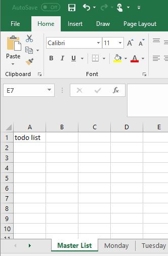
Try clicking on Master List Cell A1 ONCE, and type the words “todo List” and press enter once you are finished typing
See What Happens.
Figure 10 Activity - Data Entry
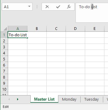
Now, DOUBLE CLICK on Cell A1 and move the cursor to the function bar as shown in figure 11 to edit the text to have correct capitalisation and hyphenation. Press Enter once you are finished editing
Figure 11 Activity - Data Editing
Now copy and paste the below table into cell A3. Only Click on Cell A3 once. Try double clicking on it, just to see what it does. Use the Undo function (CTRL+Z) to move back a step to be able to paste it again after having done a single click.
Update customer Database
simple mending of library material
shelf sorting
search for phone requests
relocation of incorrectly filed materials
Planning of current fundraising drives.
Notify borrowers of overdue materials
Interlibrary loans
Dusts or cleans materials;
Compile overdue lists
clerical tasks
Clears study tables and keeps furniture in order;
Assemble and arrange display materials.
A/V equipment audit;
You will see that the data in column A spills over into columns B, C, D and E, because column A is not wide enough to view it all. To increase the size of column A, move your mouse cursor up to the grey column reference bar and hover over the line between A and B, until your cursor changes from a pointer to a vertical line with two horizontal arrows coming off it. Once your cursor changes, double click your mouse and column A should resize automatically to fit the widest point of the text, in this case, row 14, “Clears study tables and keeps furniture in order;”
Save your work at this point, using either the quick save icon at the top of the page, or the File- Save As method explained earlier.
Adding an additional row or column:
To add a row (or a column) click on the row (or column)
AFTER the one you want to add and then right click to bring up the ‘right click
menu’. Once you have the menu visible, select “Insert”
For example, if you want to add a new blank row between row
2 and row 3, select row 3, then right click and select ‘insert’. This will move
the data in row 3 down into row 4 and leave row 3 blank.
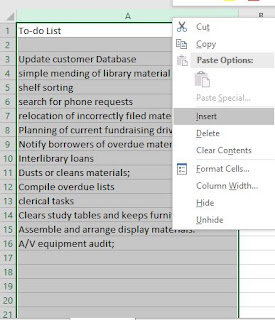
Figure 12 Insert a new row
Another example: To insert a new column before column A,
select column A, then right click and select ‘Insert’, this will move the data
in column A over into what is now column B, and leave you with a blank column A
Figure 13: Insert a new column
Activity:
In your Training Exercise:
- Add a blank column before Column A. Your list should now be sitting in column B.
- Add two blank rows above row 3. Your list should now begin in row 5
How did you go with
this activity?
Write a note in the
comments below to let us know how you are going so far.
Merge and Centre / Font Selection / Changing the Look of your text
In the last activity, the title of our list moved into Cell B2, which means it is no longer in the top left corner of our sheet.
We want to make this list title stand out on the page in addition to being anchored to the top left corner, so our next step is to make this title look like a title.
The Merge and Centre Tool
This handy-dandy tool has been introduced in the newer versions of excel, so if you are using the older versions of excel you may not have access to this feature.
On the ribbon in the Alignment group on the Home tab, you will see an icon for ‘merge & centre’, with drop down options for ‘merge across’, ‘merge cells’ and ‘unmerge cells’
Figure 14 Merge and Centre
At the beginner level you will likely only use ‘merge & centre’ and ‘unmerge’
Merging cells means to combine the cells across the width of two or more columns and/or rows. When you merge two or more neighbouring horizontal or vertical cells, the cells become one big cell that is displayed across multiple columns or rows.
Figure 15: a Merged cell surrounded by normal cells.
Important: When you merge cells, the contents of only one cell appear in the merged cell. This is the contents of the upper-left cell. The contents of the other cells that you merge will be deleted.
You can always split the merged cells later on if you change your mind. To do so, select the cells to unmerge and using the same process above, select “unmerge cells”
Activity:
In your Training Exercise:
- Select the Cells A1 through C3. (See Figure 16 for the area that should be selected)
- Use the Merge and Centre Tool to Merge these cells
Figure 16: Merge & Centre Activity
Font Size Selection
The Font group on the Home tab works much like in all other Microsoft Office products, so if you have had any exposure to Word, Outlook, Powerpoint, Publisher or Project, chances are you have seen these controls before.
To change the font size of text:
Select the text or cells with text you want to change.
Hint: (To select all text in a sheet, press Ctrl + A.)
On the Home tab, click the font size in the Font Size box.
In the font size box, you are also able to type in any size you want, between 1 and 409, in multiples of .5. So you could use size 12.5 or size 22. Or size 102 or size 202.5
Figure 17 Font Size
Activity:
- Have a play around with the size of the text in Cell A1 (The title of your table)
- How big does the size need to be before it becomes too difficult to read?
- Make a comment below to let the rest of the class know what size you tried – did you attempt size 409?
It’s also possible to change the font size using the Increase Font Size or Decrease Font Size icons (see figure 18) until the size you want is shown in the Font Size box.
Figure 18: Font size Increase Font Size
Changing the Font Colour:
In the same way as we changed the font size using the Font group on the home tab, we will use the same area to change the font colour.
Highlight the text or cells want to change.
Hint: (To select all text in a sheet, press Ctrl + A.)
On the Font group, click the arrow next to the font colour box.
Select the colour you wish to use.
Figure 19: Font Colour
Changing the Font Type
In the exact same way, the font style can be changed by selecting the font name and changing it to a different style using the font name box, located next to the font size box.
Underline, Italics, and Bold text
This is also the space where we can change the emphasis of the text by adding underline, italics or bold text types. Of note, click the drop down arrow next to the underline button to access the double underline feature.Activity:
Make your heading the following:- Font size: 22.5
- Font type: "Arial Black"
- Font colour: Red, Green or Blue (Your choice - this will influence the final look of your table)
- Emphasised Text:Double Underline
Figure 20: Title Activity
How did you go with this lesson?
There was a lot covered so let's take a break here. If there is anything you are having trouble with or would like to ask any further questions about, or just have a general comment to add, don't forget to comment below, or be in contact using the Pearl Cove email forum set up for this online course.
In LESSON FOUR: Creating and formatting a Table, using Flash Fills and predefined tables, and looking at sorting and filtering
Until next time!


